Measures of spread; shape
It is nice to have a number specifying where data lies (e.g., mean, median), but
it is also nice to know how representative of the data that number is (i.e.,
how far from that number the data lies). The data sets {10, 30, 50, 70, 90}
and
{40, 45, 50, 55, 60} both have the mean=median=midrange=50, but they differ
in how much the data is spread out. To distinguish these data sets, it is useful
to
complement a measure of location with a measure of spread or variation.
There are several statistics which
characterize the amount of spread, of which the range and the standard deviation
are most frequently used.
The range is the extent of the data set; it is defined as the maximum minus
the
minimum. For data sets A and B the range is 7 and
8,
respectively. For the weights of students the
range is 235-105=130. Note that the range is a single number, the difference
between the maximum and minimum, *not* an ordered pair specifying the minimum
and maximum. Note also that the range is defined from the extreme individuals,
hence does not measur how far a typical data value is from the middle.
If you know the midrange and range, you can calculate the maximum and minimum.
(quartiles are
defined in the next section)
The inter-quartile range is defined as Q3-Q1.
For data sets A and B the interquartile range
is 8-3 = 5 and 7-2 = 5,
respectively. Note that the inter-quartile range is a single number and not
the ordered pair consisting of the quartiles. For the weights of students the inter-quartile range is
175-130 = 45. [Different definitions for the quartiles will produce different
inter-quartile ranges.] Since Q3 is the middle of the data above the median,
and Q1 is the middle of the data below the median; Q3-Q1=(Q3-Q2)+(Q2-Q1) is
twice the average distance of a datum from the median.
Note that knowing
the median and the inter-quartile range does not let you calculate the minimum
and maximum.
Rather than the maximum extent, one might want a measure of the average distance
of data from the center
Rather than the maximum extent, one might want a measure of the average distance
of data from the center. There are several approaches to measuring the average
distance from the mean.
A first notion might be (1/n)*sum*(x(i) - x-bar),
where
there are n data points. However, it is readily verified that this quantity
is always 0, hence it is not of much use. Negative distances cancelling out
positive distances can be avoided by employing the absolute value:
(1/n)*sum*|(x(i) - x-bar)|; this quantity is called the mean
deviation
(or the mean absolute deviation).
It is a nice concept, but is not suitable for many mathematical manipulations,
hence is not widely employed.
Another way to avoid negative summands is to square them.
(1/(n-1))*sum*((x(i) - x-bar)^2) is called the variance, which is denoted by
s^2. [The reason for dividing by n-1 rather than n, is that this is the
estimate for the variance of a population based on a sample; if we had divided
by n we would have still called it the variance, but denoted it with *sigma*^2
where *sigma* is lower case sigma.] Evaluating this expression for data set
A yields ((2-5.4)^2 + (3-5.4)^2 + (5-5.4)^2 + (8-5.4)^2 + (9-5.4)^2)/4 = 9.3.
This is not a good measure of the average distance from the mean, but its
square root 3.05 is (taking the square root essentially undoes the previous
squaring). The square root of the variance is called the standard deviation,
and denoted by s. For the weights of students
the variance is 881.77, and the standard deviation is 29.69.
Exercise: In what sense is the standard deviation an average distance? How
many (what percentage) of the weights of students lie within one standard
deviation unit of the mean? Within two standard deviation units of the mean?
Within three? How many standard deviation units is the range?
To what extent do the inter-quartile range and standard deviation specify how
far data is from the center (meadian or mean)? Half the data lies between the
first and third quartile. Because data distributions are in general not
symmetric, Q1 is not equal to Q2-.5(Q3-Q1) (and Q3 is not equal to
Q2+.5(Q3-Q1)), hence we cannot say precisely what fraction of the data will lie
within one-half interqartile range of the median. But approximately half the
data will lie within one-half interquartile range of the median. [It is easy
to show that at least one-quarter of the data and at most three-quarters of the
data lies within one-half inter-quartile range of the median.]
For the standard deviation, there is no exact result either, but many data
distributions are approximately normal (for our purposes, approximately normal
means symmetric and unimodal, mound shaped). Hence we can use the exact result
for normal distributions as a rule of thumb for most data distributions:
Approximately .68 of the data (approximately 2/3) lies within one standard
deviation unit of the mean.
Approximately .95 of the data (approximately 19/20) lies within two standard
deviation units of the mean.
Approximately .9974 of the data (approximately 399/400) lies within three
standard deviation units of the mean.
[Bounds on on how much data lies within one, two, or three standrd deviation
units from the mean are available from Tchebychev's theorem, but we shall not
discuss that in this course.]
The range and standard deviation measure how
spread out data is, but do not give
any information as to how that spread is distributed among the data. We would
really like to know where all the data lies, be able to visualize a picture
like a histogram. In particular, we might want to know whether the data is
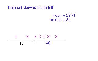
symmetric about the mean, or there is a longer tail on one side. A
distribution is said to be skewed in the direction of the longer tail. We have
seen previously that a long tail on the right side (i.e., extreme individuals
on the right not balanced by extreme individuals on the left) causes the mean
to be greater than the median. We shall employ the mean being greater than the
median as the definition of skewed to the right (although there is a more
technical defintion of skewness which does not always agree with this
definition). Similarly, if the mean is less than the median a distribution is
skewed to the left..
(Note that if a data set is symmetric the mean is equal to the median, but the
mean being equal to the median does not require that a data set be
symmetric.)
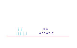
Most data distributions have a single peak, which occurs near the mean and
median; such a distribution is called unimodal. However, there are also
distributions where there are two peaks, and the mean and median lie between
them, being near neither. An example would be the weights of birds where
juveniles would be much lighter than adults resulting in some data points near
the average weight for juveniles, and other data points near the average weight
for adults. Although the weights of juveniles would be unimodal and the
weights of adults would be unimodal, the weights for the entire species would
be bimodal.
Competencies: For the data set {2 5 9 4 6 7 6 8 8}, calculate the
variance, standard deviation, and range.
Reflection: For the above data set, which of the above statistics best
describes the spread of the data?
Challenge: Is the variance always greater than the standard deviation?
When
will the variance, standard deviation, and range be equal?
May 2003
return to index
campbell@math.uni.edu